News & Events

Published On: 4/5/2022

by Drew Allmon

Blog - What’s the risk? Impacts of Parametric Assumptions for Causal Analysis of Time-to-event Outcomes

Background

Making parametric assumptions often reduces the variance of effect estimates, but by making such assumptions, the validity of the study hinges on whether those assumptions hold. The goal of this blog post is to evaluate how parametric assumptions affect the bias and variance of causal estimation of time-to-event outcomes.

Methods

To achieve this goal we conducted a simulation study to explore how non-parametric and semi-parametric estimators perform when estimating a causal risk difference. The simulated data included a binary treatment and Weibull-distributed censoring and potential outcome times. For simplicity, no covariates other than treatment were considered, though we do not anticipate the results would change in the presence of additional covariates. Two settings were assessed, one in which the hazard ratio is constant across time (proportional hazards) and one in which it is not (non-proportional hazards). The bias, variance, and mean squared error (MSE) of the risk difference estimates were assessed for each estimator.

To begin, let’s first define the data generating mechanism to use in our simulations.

#####################################################
## A: Treatment
## Y0: Failure time for controls
## Y1: Failure time for treatment group
## C: Censoring time
## Y: Observed failure time
## del: Censoring indicator (0=Censored, 1=Event)
#####################################################
dat_gen <- function(n, effect = 2, cens_shape = 2.5, p_treat = 0.5, prop_haz = TRUE) {
  tibble(
    id = 1:n,
    A = rbinom(n, 1, p_treat),
    Y0 = rweibull(n, 1, 1),
    Y1 = rweibull(n, 0.5 + 0.5 * prop_haz, effect),
    C = rweibull(n, 1, cens_shape),
    Y = pmin(A * Y1 + (1 - A) * Y0, C),
    del = Y != C
  )
}

Data were simulated in such a way to mimic realistic scenarios one might encounter in the real world. The prop_haz option indicates whether the data have proportional or non-proportional hazards. The output below gives an idea of what the data might look like for \(n=20\).

## Rows: 20
## Columns: 7
## $ id  <int> 1, 2, 3, 4, 5, 6, 7, 8, 9, 10, 11, 12, 13, 14, 15, 16, 17, 18, 19,…
## $ A   <int> 0, 0, 1, 1, 0, 1, 0, 1, 0, 1, 0, 1, 0, 0, 0, 1, 0, 1, 0, 0
## $ Y0  <dbl> 1.45669039, 0.56056998, 0.79905603, 1.08500607, 0.09342879, 0.1532…
## $ Y1  <dbl> 2.07370934, 2.44389222, 0.01335456, 2.71010207, 0.49728031, 0.9621…
## $ C   <dbl> 0.04041156, 1.90214007, 1.41779926, 2.46764865, 3.16473269, 0.2123…
## $ Y   <dbl> 0.04041156, 0.56056998, 0.01335456, 2.46764865, 0.09342879, 0.2123…
## $ del <lgl> FALSE, TRUE, TRUE, FALSE, TRUE, FALSE, TRUE, FALSE, FALSE, TRUE, T…

Estimation using Semi- and Non-Parametric Approaches

The main idea of the code below is as follows:

1. Calculate the true risk difference across a set of user-defined timepoints. We will refer to this as the ‘truth’.
2. Fit the Cox model and calculate the predicted cumulative risk at each timepoint under two scenarios: all individuals assigned treatment vs. all individuals assigned no treatment.
3. Calculate the mean of the predicted values from (2) at each timepoint by treatment group.
4. Calculate the causal risk difference at each timepoint by taking the difference in average predicted values from (3) between treatment and controls at each timepoint.
5. Use the Kaplan-Meier estimator to calculate the predicted risk at each timepoint under the scenarios from (2).
6. Calculate the mean of the predicted values from (5) at each timepoint by treatment group.
7. Calculate the causal risk difference at each timepoint by taking the difference in average predicted values from (6) between treatment and controls at each timepoint.

code_est <- function(dat, times = 1:3) {
  ## Calculate true risk difference given times of interest ##
  truth <- dat %>%
    slice(rep(1:n(), each = length(times))) %>%
    group_by(id) %>%
    mutate(time = times) %>%
    mutate(count0 = Y0 < time, count1 = Y1 < time) %>%
    group_by(time) %>%
    summarize(risk_Y0 = mean(count0), risk_Y1 = mean(count1), .groups = "drop_last") %>%
    mutate(true_risk = risk_Y1 - risk_Y0)
  
  
  ####################################### Cox Model plus Standardization ########################################################
  coxmod <- coxph(Surv(Y, del) ~ A, data = dat)
  
  ## Predict when treatment=1 for everybody ##
  preds1 <- 1 - predict(coxmod,
                        newdata = dat %>%
                          slice(rep(1:n(), each = length(times))) %>%
                          group_by(id) %>%
                          mutate(Y = times, A = 1),
                        type = "survival"
  )

  
  ## Predict when treatment=0 for everybody ##
  preds0 <- 1 - predict(coxmod,
                        newdata = dat %>%
                          slice(rep(1:n(), each = length(times))) %>%
                          group_by(id) %>%
                          mutate(Y = times, A = 0),
                        type = "survival"
  )
  
  ## Take the mean of predicted values for all n people at selected times, for both treatment groups ##
  ctp0 <- tibble(time = rep(times, nrow(dat)), A = 0, rp0 = preds0)
  c0 <- ctp0 %>%
    group_by(time, A) %>%
    summarise(r0 = mean(rp0), .groups = "drop_last")
  
  
  ctp1 <- tibble(time = rep(times, nrow(dat)), A = 1, rp1 = preds1)
  c1 <- ctp1 %>%
    group_by(time, A) %>%
    summarise(r1 = mean(rp1), .groups = "drop_last")
  
  ## Join risk for both treatment groups and calculate risk difference
  output_cox <- c0 %>%
    left_join(c1, by = "time") %>%
    mutate(rd = r1 - r0, Model = "Cox") %>%
    select(-A.x, -A.y)
  
  
  ####################################### Non-parametric ########################################################
  surv0 <- survfit(Surv(Y, del) ~ 1, data = dat %>% filter(A == 0)) ## ~1 fit intercept
  surv1 <- survfit(Surv(Y, del) ~ 0, data = dat %>% filter(A == 1)) ## ~0 no intercept
  
  s0 <- tibble(
    time = times,
    r0 = 1 - surv0$surv[findInterval(times, surv0$time)]
  ) ## Cumulative risk for A=0
  
  s1 <- tibble(
    time = times,
    r1 = 1 - surv1$surv[findInterval(times, surv1$time)]
  ) ## Cumulative risk for A=1
  
  ## Join risk for both treatment groups and calculate risk difference
  output_np <- s0 %>%
    left_join(s1, by = "time") %>%
    mutate(rd = r1 - r0, Model = "NP")
  
  results <- bind_rows(output_cox, output_np) %>%
    left_join(truth, by = "time")
}

Next, we repeat steps 1-7 for 10,000 simulations.

run_full_sim <- function(nsims, n, times, prop_haz = TRUE, seed = 123) {
  sim_results <- furrr::future_map_dfr(
    .x = 1:nsims,
    .f = function(x, n, times, prop_haz) {
      dat <- dat_gen(n, prop_haz = prop_haz)
      code_est(dat, times = times) %>%
        mutate(sim_id = x)
    },
    .options = furrr_options(seed = seed),
    n = n,
    prop_haz = prop_haz,
    times = times
  )
  
  full_truth <- sim_results %>%
    group_by(time, sim_id) %>%
    slice(1) %>% # Grabbing only 1 truth from each run, since there will be 1 for each model
    group_by(time) %>%
    summarize(
      true_r0 = mean(risk_Y0),
      true_r1 = mean(risk_Y1),
      true_rd = mean(true_risk),
      .groups = "drop_last"
    )
  
  sim_results %>%
    left_join(full_truth, by = "time") %>%
    group_by(Model, time) %>%
    summarize(
      bias_r0 = mean(r0 - true_r0),
      bias_r1 = mean(r1 - true_r1),
      bias_rd = mean(rd - true_rd),
      var_r0 = mean((r0 - mean(r0))^2),
      var_r1 = mean((r1 - mean(r1))^2),
      var_rd = mean((rd - mean(rd))^2),
      mse_r0_1 = mean((r0 - true_r0)^2),
      mse_r1_1 = mean((r1 - true_r1)^2),
      mse_rd_1 = mean((rd - true_rd)^2),
      .groups = "drop_last"
    ) %>%
    mutate(
      mse_r0_2 = bias_r0^2 + var_r0,
      mse_r1_2 = bias_r1^2 + var_r1,
      mse_rd_2 = bias_rd^2 + var_rd
    )
}

Note, the mean-squared error (MSE) was calculated using two different techniques to check for coding errors.

Results

Now we just call the function defined above for \(n=100, 500, 1000\) assuming proportional and non-proportional hazards.

results_ph_100 <- run_full_sim(10000, 100, 1:3, prop_haz = TRUE) %>% mutate(n=100)
results_ph_500 <- run_full_sim(10000, 500, 1:3, prop_haz = TRUE) %>% mutate(n=500)
results_ph_1000 <- run_full_sim(10000, 1000, 1:3, prop_haz = TRUE) %>% mutate(n=1000)
results_ph <- bind_rows(results_ph_100,results_ph_500,results_ph_1000)
results_ph <- add_column(results_ph, Assumption = "PH")

results_nonph_100 <- run_full_sim(10000, 100, 1:3, prop_haz = FALSE) %>% mutate(n=100)
results_nonph_500 <- run_full_sim(10000, 500, 1:3, prop_haz = FALSE) %>% mutate(n=500)
results_nonph_1000 <- run_full_sim(10000, 1000, 1:3, prop_haz = FALSE) %>% mutate(n=1000)
results_nonph <- bind_rows(results_nonph_100,results_nonph_500,results_nonph_1000)
results_nonph <- add_column(results_nonph,Assumption = "NonPH")

all_results <- bind_rows(results_ph, results_nonph)

Now let’s plot the information from our simulations

mynamestheme <- theme(plot.title = element_text(family = "Helvetica", face = "bold.italic", size = (15),hjust = 0.5), 
                      plot.subtitle = element_text(family = "Helvetica", face = "bold.italic", size = (12),hjust = 0.5),
                      plot.caption = element_text(family = "Helvetica", face="italic", size = (12),hjust = 0),
                      legend.title = element_text(colour = "steelblue",  face = "bold.italic", family = "Helvetica", size = (12)), 
                      legend.text = element_text(face = "italic", colour="black",family = "Helvetica", size = (12)), 
                      axis.title = element_text(face = "italic", family = "Helvetica", size = (12), colour = "black"),
                      axis.text = element_text(face = "italic", family = "Helvetica", colour = "black", size = (12)))

p1 <- ggplot(all_results,aes(time, mse_rd_1)) + geom_line(aes(colour=Model)) +
  geom_point(aes(shape=Model,colour=Model)) + 
  facet_grid(Assumption~n,labeller = "label_both") + 
  mynamestheme + theme(legend.position = "bottom") +
  labs(y="MSE",
       x="Time")

print(p1)

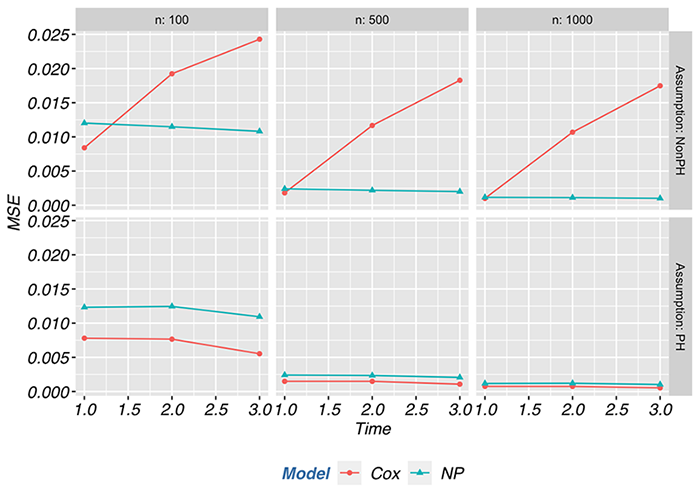
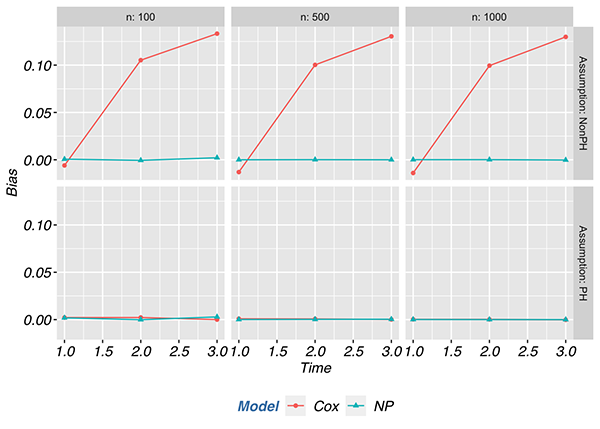
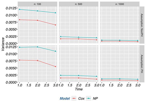
In the proportional hazards scenario, the MSE of the semi-parametric estimator was at least 50% lower compared to non-parametric estimator across most scenarios. The semi-parametric estimator had a lower MSE than the non-parametric estimator regardless of sample size when the proportional hazards assumption held. However, when the proportional hazards assumption was violated, the MSE of the semi-parametric estimator was at least twice that of the non-parametric estimator and went as high as 9.5 times the MSE with a sample size of 1000. Most of the contribution to the differences in MSE between the proportional hazards and non-proportional hazards scenarios is attributed to the bias component of MSE and not the variance. Below we depict the contributions of bias and variance to the MSE.

Conclusions

In the small set of scenarios explored here, when hazards are proportional, making parametric assumptions nearly halved the MSE compared to a non-parametric estimate. However, when the hazards were not proportional, making such assumptions at least doubled the MSE. Cole et al. (2021) perhaps said it best: “The moral of this story is an old one: It is best to be right. To be most accurate, be an”omniscient” oracle and pick the correct parametric model or rely on chance to accidentally specify the model correctly.” If you find you are not fortunate enough to be in that best case scenario, it is a good idea to use caution when your results rely on parametric assumptions.

References