News & Events

Published On: 10/19/2021

by Alex Breskin

Blog - One Model to Rule Them All: Using a Single Model to Control for Confounding and Informative Censoring

Introduction

Studies designs for estimating causal effects are numerous. Based on the design, it is often necessary to control or address several sources of bias, such as baseline and time-varying confounding, informative censoring, selection bias, and a whole host of others. Designs like the treatment decision design [1], new user design [2], and prevalent new user design [3] each address these biases in different ways and require seemingly different analytic approaches to yield unbiased estimates from their resulting data.

Recently, the ‘clone-censor-weight’ approach [4–6] has become a popular way to estimate the effects of sustained or dynamic treatment regimens. However, this approach, and the way of thinking it entails (which involves conceptualizing a ‘target trial’ and adapting it to the observational setting [7]), is more general, and nearly all studies can be thought of in this way. Here, we show that a standard study of a point treatment can be thought of as a clone-censor-weight design, and we show how confounding and informative censoring can be addressed with a single nuisance model.

The Setup

Consider a study of a binary baseline treatment, \(A\), on a time-to-event, \(T\). Patients may be censored prior to experiencing the event, and the time of censoring is \(C\). A patient’s observed follow-up time is \(\tilde{T}=min(T,C)\). In addition, a set of baseline covariates sufficient to control for confounding and informative censoring are collected, denoted \(W\). Finally, we define \(\Delta=C>\tilde{T}\), which is an indicator that a patient was not censored at their observed follow-up time (and therefore had the event). A subject’s observed data therefore consist of \(\{A, \tilde{T}, W, \Delta\}\).

One estimator for the counterfactual cumulative incidence of the outcome under treatment level \(A=a\) is [8]:

\[ \hat{Pr}(T(a)<t)=\frac{1}{n}\sum_{i=1}^n{\frac{\Delta_iI(\tilde{t}_i<t)I(A_i=a)}{\hat{Pr}(\Delta=1|W_i,A_i,T_i)\hat{Pr}(A=a|W_i)}}, \]

where \(T(a)\) is the time of the event had, possibly counter to fact, a subject received treatment level \(A=a\), \(n\) is the total population size, and each of the probabilities in the denominator are modeled appropriately, e.g., with a Cox proportional hazards model for the censoring model and logistic regression for the treatment model.

Data Generation

Here, we generate a simple dataset for demonstration.

expit <- function(p){
  exp(p)/(1+exp(p))
}

n <- 10000

dat <- tibble(
  id = 1:n,
  W = runif(n),
  A = rbinom(n, 1, expit(W)),
  T0 = rexp(n, rate = 0.5 + 2*W),
  T1 = rexp(n, rate = 1 + 2*W),
  T = A*T1 + (1-A)*T0,
  C = rexp(n, rate = .5 + .55*A + .5*W)
)

Note that our true causal risk difference is 11.93%.

Typical Study Design and Analysis

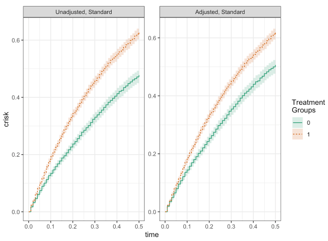
Using the causalRisk package, we can easily implement the estimator described above to get the unadjusted and adjusted cumulative incidence curves:

mod_unadj <- specify_models(identify_treatment(A),
                            identify_outcome(T),
                            identify_censoring(C))

mod_adj <- specify_models(identify_treatment(A, ~W),
                          identify_outcome(T),
                          identify_censoring(C, ~W))

fit_unadj <- estimate_ipwrisk(dat, mod_unadj, times = seq(0, 0.5, by = 0.01), labels = "Unadjusted, Standard")

fit_adj <- estimate_ipwrisk(dat, mod_adj, times = seq(0, 0.5, by = 0.01), labels = "Adjusted, Standard")

make_table1(fit_adj, side.by.side = T)

plot(fit_unadj, fit_adj)

make_table2(fit_unadj, fit_adj, risk_time = 0.5)

Clone-Censor-Weight Design with Single Model

While the previously described analysis seems to work fine, it is limited by the fact that treatment must occur at a single point in time. The clone-censor-weight design relaxes this restriction by allowing for sustained treatments or dynamic treatment regimens. This is accomplished by a 3-step process:

1. ‘Clone’ each patient once for each treatment regimen of interest.
2. ‘Censor’ each clone when their person-time is no longer consistent with the corresponding treatment regimen.
3. ‘Weight’ the remaining person-time by the inverse probability of being censored.

This approach is quite general and can easily accommodate simple study designs like the one previously undertaken here. One complicating factor, however, is the need to handle baseline as well as time-varying treatment. The 3-step process does not seem to have any way of dealing with baseline treatment, for instance using inverse probability of treatment weights. Doing so would require, within each set of ‘clones’, further dividing the clones by baseline treatment and applying both treatment and censoring weights.

It turns out that a single Cox proportional hazards model can be used to handle baseline and time-varying treatments. This is accomplished by ensuring that all patients contribute at least some person-time (so patients who are on the ‘wrong’ treatment at baseline are given some tiny amount of person-time) and specifying the censoring model flexibly enough to act as if it were in fact two separate models - one for treatment and one for censoring.

Here, we demonstrate how this works.

dat2_treat <- dat %>%
  group_by(id) %>%
  mutate(C2 = ifelse(A == 0, runif(n, min = 1e-8, max = 1e-7), C)) %>%
  slice(rep(1, 2)) %>%
  mutate(t_ind = ifelse(row_number() == 1, 1, 0),
         end = ifelse(row_number() == 1, 1e-7, C2),
         start = ifelse(row_number() == 1, 0, lag(end))) %>%
  filter(start != end) %>%
  mutate(treat = 1) %>%
  mutate(del = ifelse(row_number() == n(), 1, 0)) %>%
  mutate(end = ifelse(end > .5, .5, end),
         del = ifelse(end >= .5, 0, del)) %>%
  ungroup()

dat2_notreat <- dat %>%
  group_by(id) %>%
  mutate(C2 = ifelse(A == 1, runif(n, min = 1e-8, 1e-7), C)) %>%
  slice(rep(1, 2)) %>%
  mutate(t_ind = ifelse(row_number() == 1, 1, 0),
         end = ifelse(row_number() == 1, 1e-7, C2),
         start = ifelse(row_number() == 1, 0, lag(end))) %>%
  filter(start != end) %>%
  mutate(treat = 0) %>%
  mutate(del = ifelse(row_number() == n(), 1, 0)) %>%
  mutate(end = ifelse(end > .5, .5, end),
         del = ifelse(end >= .5, 0, del)) %>%
  ungroup()

dat2 <- bind_rows(dat2_treat, dat2_notreat)

mod_ccw <- specify_models(identify_treatment(treat),
                          identify_outcome(T),
                          identify_censoring(C2, ~W + W:t_ind),
                          identify_interval(start, end),
                          identify_subject(id))

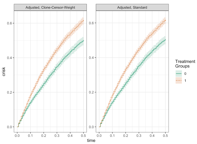
fit_ccw <- estimate_ipwrisk(dat2, mod_ccw, times = seq(0, 0.5, by = 0.01), labels = "Adjusted, Clone-Censor-Weight")

plot(fit_ccw, fit_adj)

make_table2(fit_ccw, fit_adj, risk_time = 0.5)

Conclusion

As you can see, besides a bit of numerical noise, the results from the two approaches are essentially the same! From this simple example, we can see how the clone-censor-weight design may be able to provide a general framework for the types of studies typically encountered in epidemiology.

References